1. Introduction: Supervised learning is not enough to bring out full potential of ViT
"Self-supervised learning is the cake, supervised learning is the icing on the cake, and reinforcement learning is the cherry on the cake." — Yann LeCun
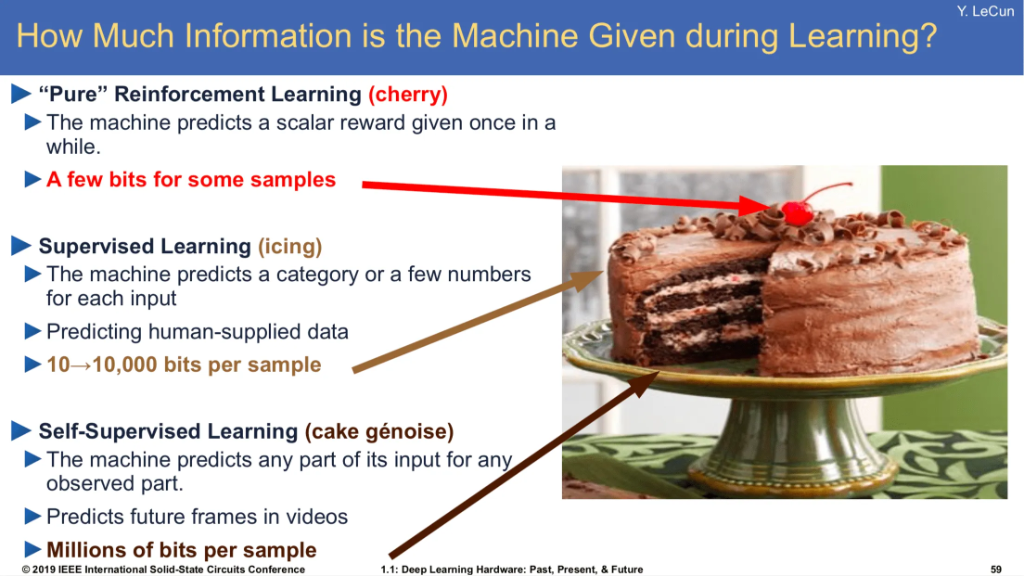
The "Cake" Analogy: SSL provides dense feedback signal (millions of bits) compared to sparse rewards in RL.
1.1 The Context: The "Data Hungry" Challenge
When Vision Transformer (ViT) was first introduced (Dosovitskiy et al., 2021), it faced three hurdles preventing it from simply replacing CNNs:
- Lack of Inductive Bias: CNNs have built-in "assumptions" about images (locality, shift invariance). ViTs, treating images as generic sequences, must learn these spatial rules from scratch, making them extremely data-hungry.
- Rugged Optimization Landscape: Without these priors, ViTs are notoriously hard to optimize. Training from scratch on standard datasets (like ImageNet-1k) often leads to overfitting or unstable convergence compared to ResNets.
- Signal Sparsity: Supervised Learning gives a "weak" signal (one integer label per image). For a model as flexible as ViT, this scalar feedback is insufficient to constrain the massive parameter space effectively. They need "dense" supervision—which is exactly what Self-Supervised Learning (SSL) provides.
Enter Self-Supervised Learning (SSL): As Yann LeCun's "Cake" analogy suggests, supervised learning (labels) limits the information signal. SSL provides a dense signal that allows ViT to learn these structural rules from the data itself, without needing 300M human labels.
Before DINO, SSL was dominated by Contrastive Learning:
- Contrastive Learning: Push positive pairs (views of same image) together, push negative pairs (different images) apart.
- The Limitation: Requires large batch sizes or memory banks for negative samples to be effective.
Distillation approaches (like BYOL) emerged to remove the need for negative pairs, relying only on positive pairs. DINO (2021) took this further by integrating it with Vision Transformers (ViTs).
1.2 The Genealogy of DINO
- DINO (2021): "Emerging Properties in Self-Supervised Vision Transformers". Proved ViTs can learn unsupervised segmentations.
- DINOv2 (2023): "Learning Robust Visual Features without Supervision". Scaling up data and combining objectives (iBOT) for a universal backbone.
- DINOv3 (2025): "A Vision Transformer for Every Use Case". Solving the "dense feature degradation" problem in long training runs using Gram Anchoring.
2. DINO (v1): Self-Distillation with NO Labels
Core Idea: If we treat the same network as both a "Teacher" and a "Student", can the student learn from the teacher's output without collapsing to a trivial solution?
2.1 High-Level Concept
The core idea is self-distillation. A student network is trained to match the output distribution of a teacher network. The key is that the teacher network's weights are not learned through backpropagation; instead, they are a "momentum" version of the student's weights, which provides a more stable learning target.
2.2 Network Architecture
-
Student Network (): This is the main network being trained. It consists of a backbone (like a Vision Transformer or ViT) and a projection head (an MLP). Its weights, , are updated via backpropagation.
-
Teacher Network (): This network has the exact same architecture as the student. Its weights, , are not updated by the optimizer. Instead, they are an exponential moving average (EMA) of the student's weights.
2.3 The DINO Algorithm: Step-by-Step
Here is the process for a single training step:
Step 1: Data Preparation (Multi-Crop Augmentation)
From a single input image (e.g., a photo), the algorithm generates a "batch" of different views. This batch is split into two main categories:
- Global Views (The "Teacher's" View):
- What they are: Two separate, large crops are taken from the original image.
- Process: The algorithm randomly selects a large area (e.g., 50% to 100% of the original image) and a random aspect ratio. This crop is then resized to the network's standard input size (e.g., pixels). There will be a meaningful amount of overlap between two images.
- Purpose: These views contain the overall scene and context—the "big picture."
- Local Views (The "Student's" Test):
- What they are: Several (e.g., 4, 6, or 8) additional, small crops are taken.
- Process: The algorithm randomly selects very small areas (e.g., 5% to 40% of the original image). These tiny crops are then resized to a much smaller input size (e.g., pixels).
- Purpose: These views act as "zoomed-in" details, like looking at just an eye, a wheel, or a single leaf.
The Augmentation Pipeline
Crucially, every single crop (both global and local) is passed through a strong data augmentation pipeline to make the task harder and prevent the model from "cheating" by just memorizing simple colors or textures. This pipeline includes:
- Random Resized Crop: This is the multi-crop process itself.
- Random Horizontal Flip: Flips the image with a 50% probability.
- Color Jitter: Randomly changes the image's brightness, contrast, saturation, and hue.
- Gaussian Blur: Randomly applies a blur to the image.
- Solarization: A strong augmentation that inverts the pixel values above a certain threshold.
By the end of this step, you have a set of highly varied, distorted images. The student network is then given the difficult task (in Step 5) of proving that a tiny, blurred, solarized local view (like a patch of fur) belongs to the same global concept as the large, global view of the whole animal. This forces it to learn what "fur" is in a general sense, rather than just memorizing a specific patch.
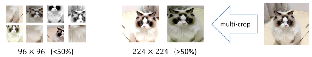
DINO Multi-Crop Strategy: 2 Global crops (>50%) cover the scene, while multiple Local crops (<50%) capture details. The student must match the teacher's global view from only a local view.
Step 2: Forward Pass
The crops are passed through the networks differently:
- All crops (both global and local) are fed into the student network .
- Only the two global crops are fed into the teacher network .
This "local-to-global" strategy forces the student to learn global information even when it's only looking at a small patch.
Step 3: Avoiding Collapse (Centering & Sharpening)
Before calculating the loss, the network outputs are processed to prevent "model collapse" (where the network outputs the same thing for every input).
-
Teacher Output (Sharpening): The teacher network's -dimensional output is passed through a
softmaxfunction with a very low temperature (e.g., 0.04). This "sharpens" the probability distribution, making it more peaked and preventing collapse to a uniform distribution.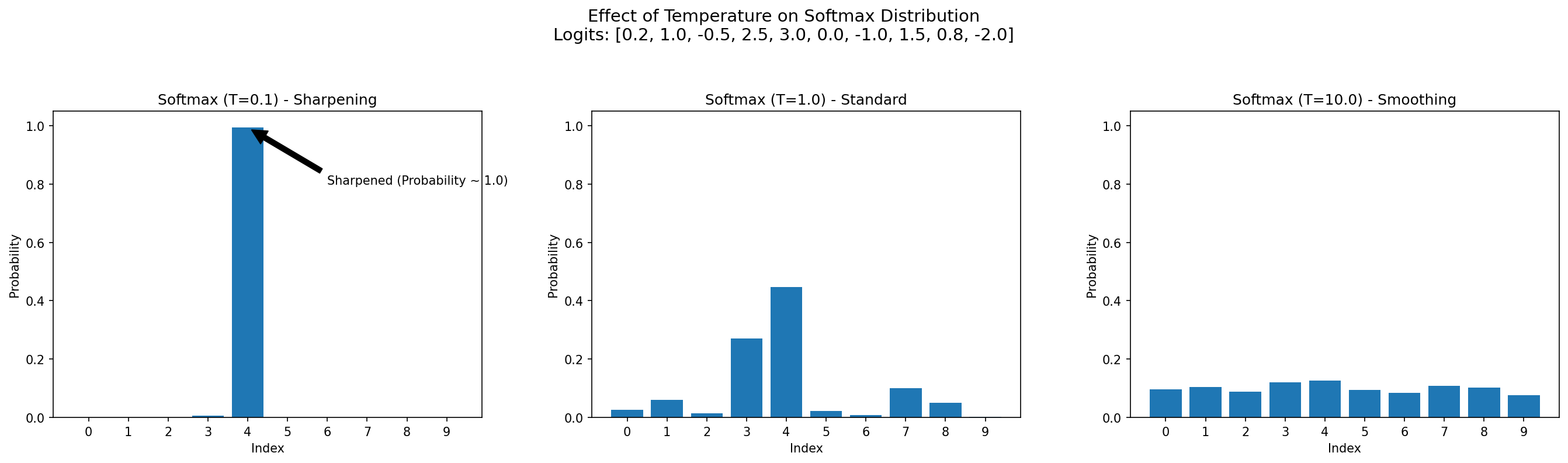
Effect of Temperature on Softmax: Lower temperature (T=0.1) creates a sharper distribution (peaked), acting as a pseudo-label for the student.
-
Teacher Output (Centering): The teacher's outputs are "centered" by subtracting a moving average of the outputs from the entire batch. This center is also updated using an EMA. This prevents a single dimension from dominating the output.
-
Student Output: The student's -dimensional output is passed through a
softmaxwith a higher temperature (e.g., 0.1).
Step 4: Loss Calculation (Cross-Entropy)
The goal is to make the student's output distribution, , match the teacher's centered and sharpened output distribution, .
This is done by minimizing a cross-entropy loss:
In plain English:
- For each crop fed through the student, its output is compared against both global teacher outputs ( and ).
- The total loss is the average of all these cross-entropy comparisons.
A stop-gradient (sg) is applied to the teacher's output, so the gradient only flows back through the student network.
Step 5: Weight Update
Two different updates happen at the end of the step:
-
Student Weights (): The student's weights are updated using backpropagation and an optimizer (like SGD) based on the loss calculated in the previous step.
-
Teacher Weights (): The teacher's weights are updated as an EMA of the student's newly updated weights:
The parameter is a momentum schedule that slowly increases from a value like 0.996 up to 1 during training, making the teacher's updates gradually "freeze".
2.4 Mathematical Detail: Algorithm Summary

DINO Algorithm Animation: Visualizing the self-distillation process.
2.5 Performance Evaluation
The DINO paper evaluates the model using two primary classification metrics on ImageNet:
-
Linear Probe:
- Protocol: Freeze the backbone (weights are fixed). Train a single linear layer (Logistic Regression) on top of the features for classification.
- Meaning: Measures "Linear Separability". It asks: "Are the features arranged simply enough that a straight line can separate cats from dogs?"
-
-NN Classifier:
- Protocol: Freeze the backbone. For a test image, compare its feature vector to all training images using Cosine Similarity. The class is determined by a vote of the nearest neighbors.
- Meaning: Measures "Manifold Structure". It asks: "Do images of the same class naturally clump together in the feature space without any supervisory training?"
-
Throughput (im/s): How fast the model processes images (images per second).
Key Findings (from Table 2):
| Method | Arch. | Param. | im/s | Linear | -NN |
|---|---|---|---|---|---|
| ResNet-50 | |||||
| Supervised | RN50 | 23 | 1237 | 79.3 | 79.3 |
| SCLR | RN50 | 23 | 1237 | 69.1 | 60.7 |
| MoCov2 | RN50 | 23 | 1237 | 71.1 | 61.9 |
| BYOL | RN50 | 23 | 1237 | 74.4 | 64.8 |
| SwAV | RN50 | 23 | 1237 | 75.3 | 65.7 |
| DINO | RN50 | 23 | 1237 | 75.3 | 67.5 |
| ViT-Small | |||||
| Supervised | ViT-S | 21 | 1007 | 79.8 | 79.8 |
| BYOL* | ViT-S | 21 | 1007 | 71.4 | 66.6 |
| MoCov2* | ViT-S | 21 | 1007 | 72.7 | 64.4 |
| SwAV* | ViT-S | 21 | 1007 | 73.5 | 66.3 |
| DINO | ViT-S | 21 | 1007 | 77.0 | 74.5 |
| Cross-Architecture | |||||
| DINO | ViT-B/16 | 85 | 312 | 78.2 | 76.1 |
| DINO | ViT-S/8 | 21 | 180 | 79.7 | 78.3 |
| DINO | ViT-B/8 | 85 | 63 | 80.1 | 77.4 |
- ViT vs. ResNet: DINO works best with Vision Transformers. While it matches methods like SwAV on ResNet-50 (75.3%), it significantly outperforms them when using ViT architectures.
- The Patch Size Trade-off:
- ViT-S/16 (Standard 16x16 patches): High speed (1007 im/s) with decent accuracy (77.0%).
- ViT-S/8 (Smaller 8x8 patches): Significant accuracy boost (79.7% Linear, 78.3% k-NN) but much slower speed (180 im/s).
- Correction on "Batch Size": The performance gain comes from smaller Patch Size (finer granularity), not smaller Batch Size. Smaller patches typically improve accuracy but quadratically increase computational cost.
- -NN Performance: DINO achieves remarkably high -NN accuracy (78.3% with ViT-S/8), suggesting the embedding space is highly structured and semantically meaningful even without any classifier training.
2.6 Emerging Properties
DINO v1 revealed something magical: Self-Attention maps automatically segment objects.
- In supervised training, the CLS token focuses on discriminative parts (e.g., the dog's ear).
- In DINO, the attention maps cover the entire object, effectively performing unsupervised segmentation.
3. DINOv2: Learning Robust Visual Features without Supervision
Motivation: While DINO v1 showed the potential of SSL, it was trained on ImageNet (curated). Scaling it to uncurated Internet data (like CLIP) proved difficult—data quality became the bottleneck. DINOv2 addresses this by building a customized, automated data curation pipeline to create a "Vision Foundation Model" that works out-of-the-box for both semantic (classification) and geometric (segmentation/depth) tasks.
3.1 Data is King: The LVD-142M Algorithm
The authors found that simply adding more uncurated data doesn't guarantee better performance. Instead, they built a sophisticated pipeline to curate the LVD-142M dataset (Large Visual Data, 142M images).
Here is the flow of their "Data Engine":
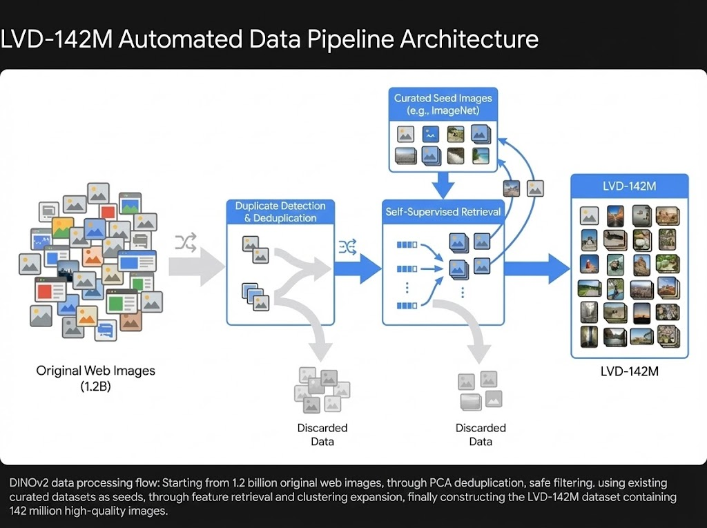
- Source: Started with 1.2 billion raw images crawled from the web (filtering out NSFW and identifiable metrics).
- Copy Detection: Removed near-duplicates to prevent memorization and redundancy.
- Self-Supervised Retrieval:
- They used a frozen ViT-H trained on ImageNet-22k to compute embeddings for all 1.2B images.
- They then retrieved images that were semantically similar to curated datasets (like ImageNet-22k and Google Landmarks). This acts as a "soft filter"—keeping web images that look like "real objects" or "clean scenes" while discarding random noise.
- Clustering & Rebalancing: They clustered the retrieved images and re-sampled them to ensure a balanced distribution, preventing the model from overfitting to dominant concepts.
3.2 Methodological Upgrades
DINOv2 combines the best parts of DINO and iBOT (masked image modeling) into a unified objective.
系统数据流向图
-
Image-Level (DINO): The student matches the teacher's global class token output. Learns high-level semantics.
where and represent the probability distributions (Softmax outputs) of the teacher and student networks, respectively.
-
Patch-Level (iBOT): Some patches are masked. The student must reconstruct the teacher's features for these masked patches. Learns low-level structure.
where is the set of masked indices, and are teacher and student outputs, and represents the masked view input to the student.
-
Untying Head Weights: Crucially, DINOv2 uses separate projection heads for DINO and iBOT losses, unlike previous works that shared them. This prevents conflict between the two objectives.
-
KoLeo Regularizer: A new loss term based on differential entropy. It forces feature vectors in a batch to be uniformly distributed on the hypersphere, preventing collapse and ensuring the embedding space is fully utilized. Some simple demo examples can be found in this github repo (opens in a new tab).
where is the batch size, is the feature vector of the -th sample, and the term minimizes the distance to the nearest neighbor () for each sample.
-
High-Resolution Adaptation: A final, short training phase increases the resolution (e.g., to ). This is crucial for dense prediction tasks like segmentation.
3.3 Scaling Engineering (ViT-Giant)
Training a 1.1 Billion parameter (ViT-Giant) model requires massive optimization:
- FlashAttention: Used to speed up self-attention and reduce memory usage.
- Sequence Packing: Instead of padding sequences to the same length (wasteful) or using nested tensors (complex), they concatenate all sequences into one long buffer and use block-diagonal attention masks. This drastically improves efficiency for multi-crop training where crop sizes vary.
- FSDP (Fully Sharded Data Parallel): Splits model parameters, gradients, and optimizer states across GPUs, allowing the giant model to fit into memory.
3.4 Evaluation: The "Frozen Features" Philosophy
DINOv2's core evaluation metric is the performance of Frozen Features—using the pre-trained backbone without any fine-tuning. This tests the model's "out-of-the-box" capability as a true Foundation Model.
1. Quantitative Benchmarks
The model achieves state-of-the-art results across diverse tasks using simple heads on frozen features:
| Task | Metric | Performance | Comparison |
|---|---|---|---|
| ImageNet Classification | Top-1 Acc | 86.5% | Matches weakly-supervised SotA (e.g., OpenCLIP-G) and beats iBOT. |
| Semantic Segmentation | ADE20k mIoU | 53.0% | Outperforms many supervised baselines; DINOv2+Mask2Former reaches 60.2%. |
| Depth Estimation | NYUd RMSE | 0.298 | Excellent reasoning of 3D geometry from 2D images. |
| OOD Robustness | ImageNet-A | High | ~20-30% improvement over iBOT on adversarial/sketch domains. |
[!TIP] Which embedding should you use?
- Global Tasks (Classification, Retrieval): Use the
[CLS]token (or average pool). It aggregates global semantics.- Dense Tasks (Segmentation, Depth): Use the Patch Tokens. Thanks to the iBOT objective, these tokens preserve precise spatial information.
2. Qualitative Capabilities
-
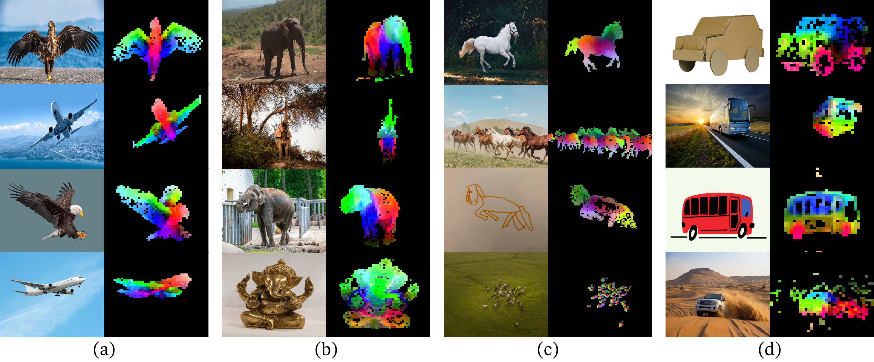
PCA Visualization: Principal Component Analysis of the feature maps shows that semantic parts (e.g., bird heads, wheel spokes) are automatically aligned across different images without any supervision.
-
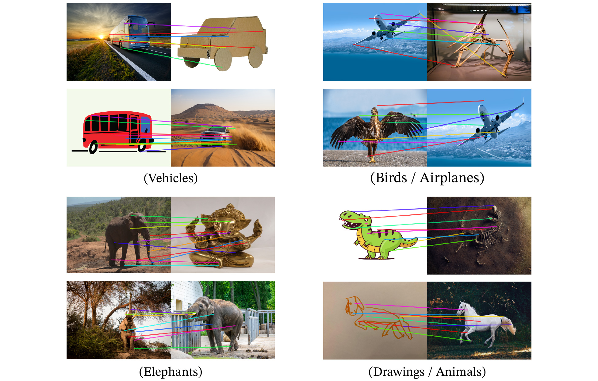
Instance Retrieval & Matching: On Oxford/Paris datasets, standard cosine similarity retrieval works out-of-the-box. As shown below, features can match similar semantic parts (wings, wheels) across vastly different poses and styles (e.g., photo vs drawing).
4. DINOv3: The "Infinite Training" Paradox
4.1 The Paradox: Global Gain, Local Pain
DINOv3 (2025) uncovered a surprising phenomenon: longer training doesn't always mean better features.
When scaling DINOv2 to larger data and longer schedules:
- Global Metrics (e.g., ImageNet Classification): Continue to improve indefinitely. The model learns better invariant semantics (e.g., "this is a dog").
- Dense Metrics (e.g., Segmentation, Depth): Peak early (~200k iterations) and then consistently degrade. The model becomes too abstract, losing the spatial coherence needed to say where the dog is pixel-by-pixel.
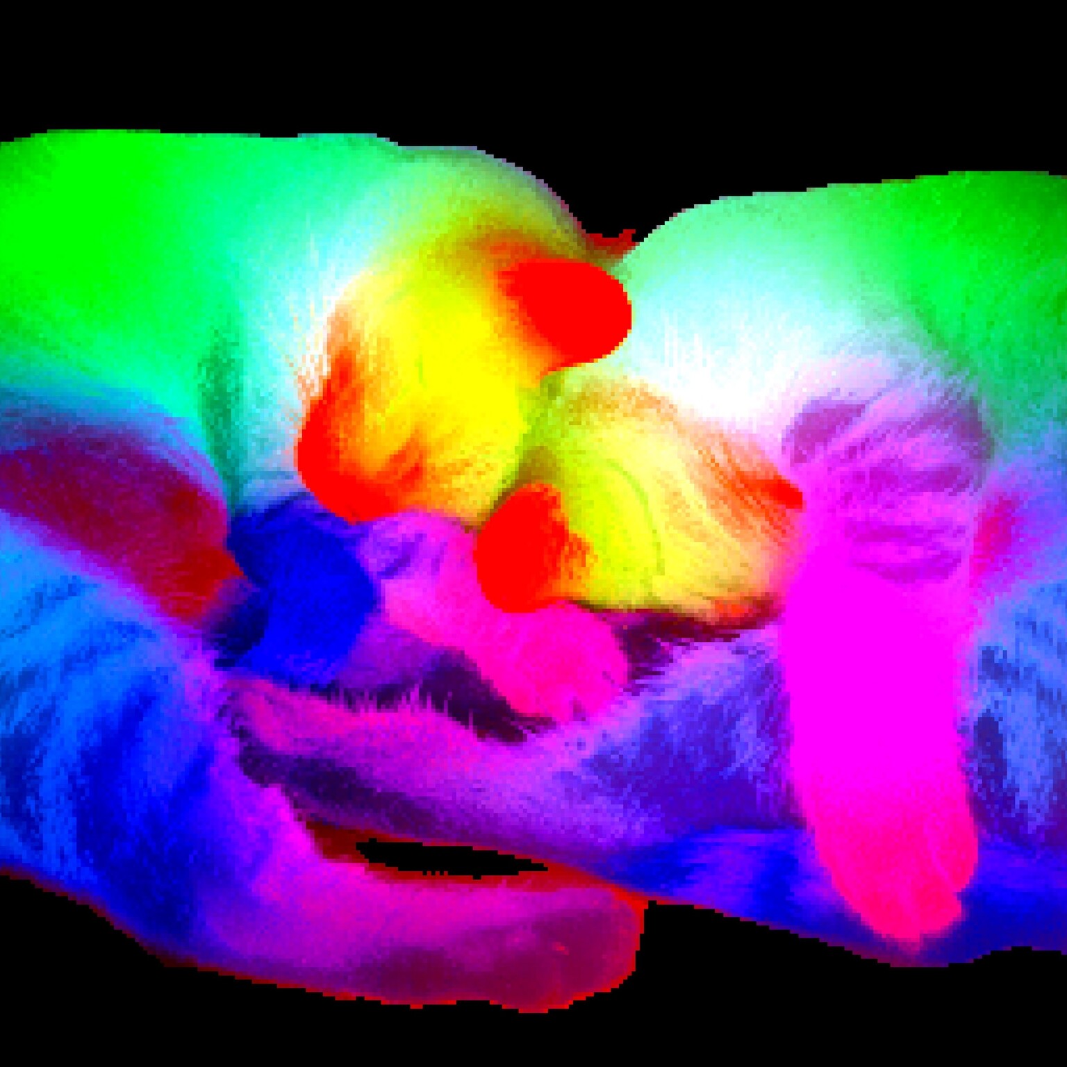
Visualizing the Collapse: Below, we observe the "Infinite Training Paradox" through two lenses:
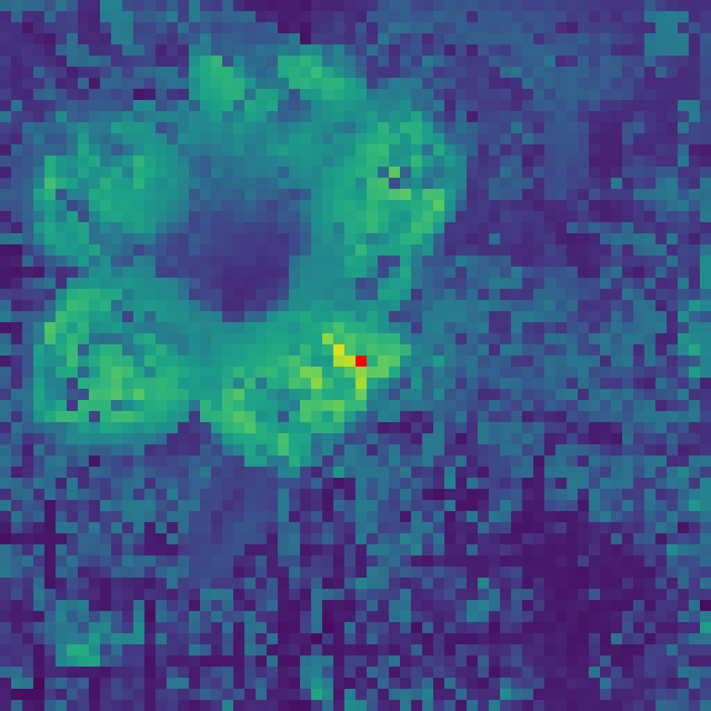
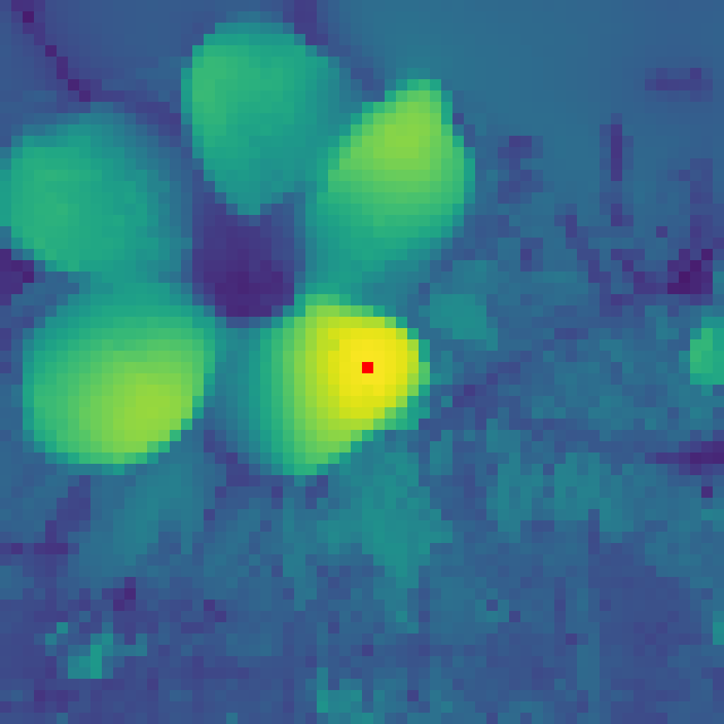
- Visual (Top Row): Feature maps of a specific patch (red dot) at 200k, 600k, and 1M iterations. Note how the attention starts clean but degenerates into background noise.
- Statistical (Bottom Row): Performance curves showing the divergence. While ImageNet accuracy (Pink) rises, dense task performance (Blue) crashes.
Exhibit A: Visual Collapse (Attention Maps)
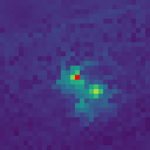
200k Iterations (Peak)
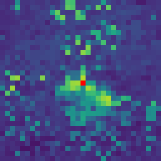
1M Iterations (Collapsed)
Exhibit B: Statistical Divergence (Performance)
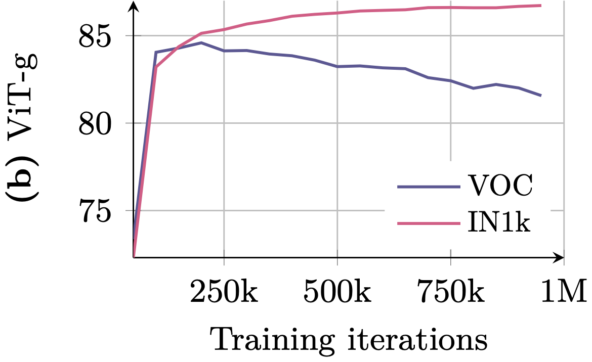
ViT-g: ImageNet (Pink) rises, but VOC (Blue) degrades after 200k.
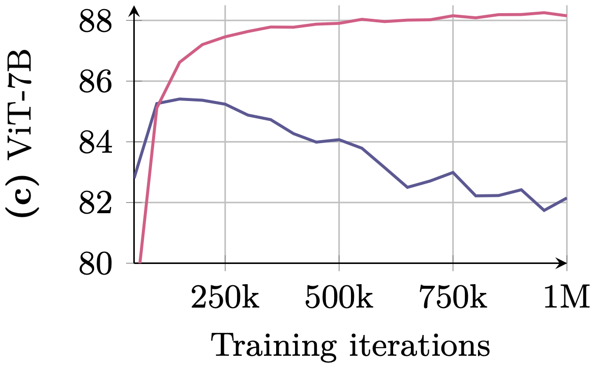
ViT-7B: Dense performance (Blue) collapses while global metrics stay stable.
4.2 The Solution: Gram Anchoring
To solve this, DINOv3 introduces Gram Anchoring, a regularization technique that acts as a "structural anchor."
The "Gram Teacher"
The idea is simple: interpret the Gram Matrix of the features as a "fingerprint" of the image's geometry/texture.
- Snapshot: Take a "Gram Teacher" from an early, healthy stage of training (or use high-res inputs).
- Regularize: Force the student model (which is learning advanced semantics) to maintain the same patch-to-patch relationships as the Gram Teacher.
This allows the feature values to evolve (improving classification) while "anchoring" their structure (preserving segmentation).
Effect of Gram Anchoring: Comparing features trained without (Left) vs with (Right) Gram Anchoring. The anchored model preserves sharp, object-aligned boundaries.
Without Gram (Noisy)
With Gram (Anchored)
4.3 High-Resolution Refinement
A key trick in DINOv3 is using High-Resolution input for the Gram Teacher.
- The Student sees a standard image.
- The Gram Teacher sees a version.
- The Gram Matrix forces the student to "hallucinate" the structural coherence of the high-res image, effectively distilling high-res quality into a standard-res model.
4.4 Final Results
The result is a 7B parameter frozen backbone that achieves state-of-the-art results on both ends of the spectrum.
DINOv3 PCA Visualization: Sharp, semantic coherency even in complex scenes.
- Scalability: Solves the degradation paradox, enabling training on 17B images (LVD-1689M).
- Performance: Sets SOTA for Semantic Segmentation (ADE20k) and Monocular Depth, purely with frozen features.
5. Visual Summary & Conclusion
5.1 Evolution Table
| Feature | DINO (v1) | DINOv2 | DINOv3 |
|---|---|---|---|
| Year | 2021 | 2023 | 2025 |
| Core Method | Self-Distillation | DINO + iBOT (MIM) | DINO + iBOT + Gram Anchoring |
| Collapse Prevention | Centering + Sharpening | Sinkhorn-Knopp + KoLeo | Same + Gram Regularization |
| Data | ImageNet (1M) | LVD-142M (Curated) | Scaled & Long-schedule |
| Main Strength | Unsupervised Segmentation | Robust Generalist Features | Infinite Training Stability |
| Weakness | Hard to scale to web data | Dense features degrade if trained too long | Complexity of multiple teachers |
5.2 Takeaway
The DINO series represents the shift from Contrastive to Generative/Distillative learning in Vision.
- v1 taught us that simple rules (centering/sharpening) yield emergent intelligence.
- v2 taught us that Data Quality matters as much as the algorithm.
- v3 taught us that maximizing one metric (global loss) can hurt others (dense consistency), and we need Explicit Structural Regularization (Gram Anchoring) to balance them.
5.3 Further Reading
- DINOv1 Paper (opens in a new tab)
- DINOv2 Paper (opens in a new tab)
- DINOv3 Paper (opens in a new tab)