import Comments from '../../components/Comments'

Introduction

Diffusion model has proven to be a very powerful generative model and achieved huge success in image synthesis. One of the most widely known application is the synthesis of images condition on text or image input. Models like ... take one step further to generate short videos based on instruction.

Meanwhile extending this power model to 3D is far from trivial. It can be represented in point, voxel, surface and etc. Unlike image data, all these forms are less structured and should be invariant w.r.t. permutation. Each of the above data structures requires different techniques to deal with(i.e. PointNet for point cloud, graph neural network for surface data etc).

Point-Voxel diffusion

Direct application of diffusion models on either voxel and point representation results in poor generation quality. The paper Zhou et al. proposed Point-Voxel diffusion(PVD) that utilize both point-wise and voxel-wise information to guide diffusion. The framework is almost exactly the same as DDPM except for the choice of backbone network. Instead of using U-Net to denoise, the paper applied point-voxel CNN to parameterize their model. Point-voxel CNN is capable of extract features from point cloud data and requires much less computational resource than previous methods(i.e. PointNet).

Quick review of DDPM

Here, we quickly review the training and sampling process with diffusion model. The DDPM parameterize the model learn the "noise" ${ϵ}_{\theta }(x_t,t)$ and the paper used a point-voxel CNN to represent ${ϵ}_{\theta }(x_t,t)$. The loss function is

WIth a trained model ${ϵ}_{\theta }(x_t,t)$, the sampling process is

where $z\sim \mathcal{N}(o,I)$.

In the context of this paper, $x_0\in {\mathbb{R}}^{N\times 3}$ is point cloud data.

Experiment

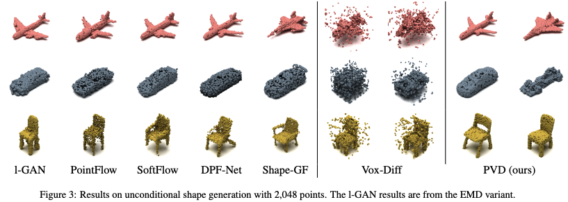
In the experiment part, the paper tested the algorithm on tasks of shape generation and shape completeion. It examined metrics such as Chamfer Distance(CD) (opens in a new tab), Earth Mover's Distance(EMD) (opens in a new tab) and etc.

Diffusion Probabilistic Models for 3D Point Cloud Generation(DPM)

The paper Luo and Hu proposed a framework that introduced latent encoding to the DDPM. The diffusion process and reverse process still happens in physical space, not in latent space. The latent variable is used as a guidence during the reverse process.

For clarity of discussion, we denote $\mathbf{X}=\{x_i{\}}_{i\in [N]}$ to be a 3D shape in the form of point cloud and $x_i\in {\mathbb{R}}^3$ for $i\in [N]$ represents each point in the point cloud. Let $\tilde{p}(\mathbf{X})$ be the distribution of shapes $\mathbf{X}$ and $p(x)$ be the distribution of points in arbitrary shapes.

Formulation

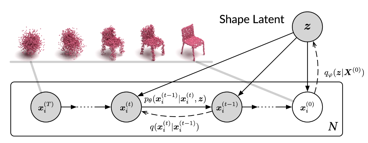
The paper introduced a latent variable $\mathbf{z}\sim q_{\phi }(\mathbf{z}\mid {\mathbf{X}}^{(0)})=\mathcal{N}\left(z\mid {\mu }_{\phi }({\mathbf{X}}^{(0)},{\Sigma }_{\phi }({\mathbf{X}}^{(0)}))\right)$. However, instead of apply diffusion process in latent space as in Rombach et al., it is used only as a guidence during the diffusion ${\mathbf{X}}^{(t-1)}\sim p_{\theta }(\cdot \mid {\mathbf{X}}^{(t)},\mathbf{z})$. More importantly, unlike PVD or image-based diffusion model, the diffusion process is conducted pointwisely. To be more specific, each point in a point cloud is diffused separately $x_i^{(t-1)}\sim p_{\theta }\left(\cdot \mid x_i^{(t)},z\right)$. The paper further concluded that points in a given point cloud is conditionally independent(given the point cloud/shape) and, mathematically, can be formulated as

This is also shown in the following graphical model.

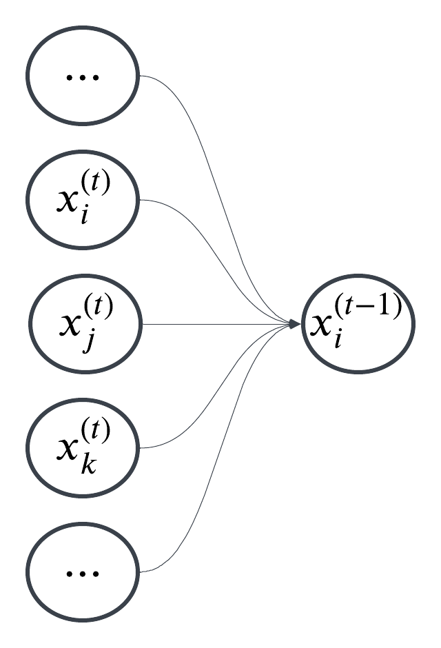
In comparison, the PVD update each reverse diffusion step through updating all points simutaniously and can be viewed as following graphical model.

The forward process is the same as DDPM or PVD which is simply adding noise to the points. The reverse process is formulated as

In this setup, $p_{\theta }(x^{(0)})$ represent an image's probability under the learned model $p_{\theta }$ and, in below, we will use $q_{\phi }(z\mid {\mathbf{X}}^{(0)})$ as the encoder. For simplicity of discussion, we will use $p_{\theta }$ to replace ${\tilde{p}}_{\theta }$.

Training objective

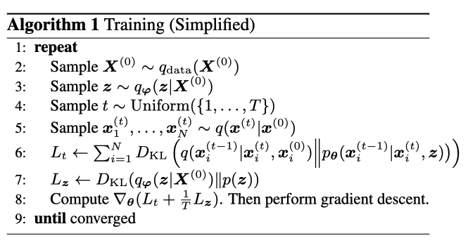
Similar to DDPM, the log-likelihood of reverse process $p_{\theta }(x^{(0)})$ can be lower bounded by

The process is parameterized by $\theta ,\phi$ and the variational lower bound can be written into KL divergencies,

This objective function can be then written in the form of points(instead of shapes) as follows,

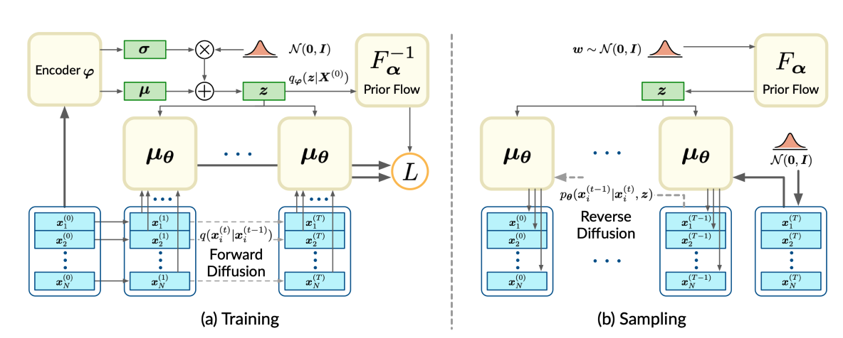
Another important point about this paper is that it does not assume the prior distribution of the latent variable $z$ to be standard normal. Instead, the algorithm needs to learn the prior distribution for sampling. Therefore, both side of $D_{\mathrm{KL}}\left(q_{\mathbf{\phi }}\left(\mathbf{z}\mid {\mathbf{X}}^{(0)}\right)\Vert p(\mathbf{z})\right)$ involves trainable parameters. An encoder $q_{\mathbf{\phi }}\left(\mathbf{z}\mid {\mathbf{X}}^{(0)}\right)$ is learned by parameterizing it with ${\mathbf{\mu }}_{\phi }\left({\mathbf{X}}^{(0)}\right),{\mathbf{\Sigma }}_{\mathbf{\phi }}\left({\mathbf{X}}^{(0)}\right)$. An map $F_{\alpha }$ that transform samples in standard normal to prior distribution is learned by parameterizing it with a bijection neural network and $z=F_{\alpha }(\omega )$.

Latent Point Diffusion Models(LION)

The latent diffusion model Rombach et al. in image synthesis conducted the diffusion process in the latent space. The paper Vahdat et al., unlike previously mentioned PVD, applied the similar spirit to the 3D point clouds.

Formulation

The model is consist of a VAE to encode shapes to latent space and diffusion models that map vectors from standard normal distribution to latent space.

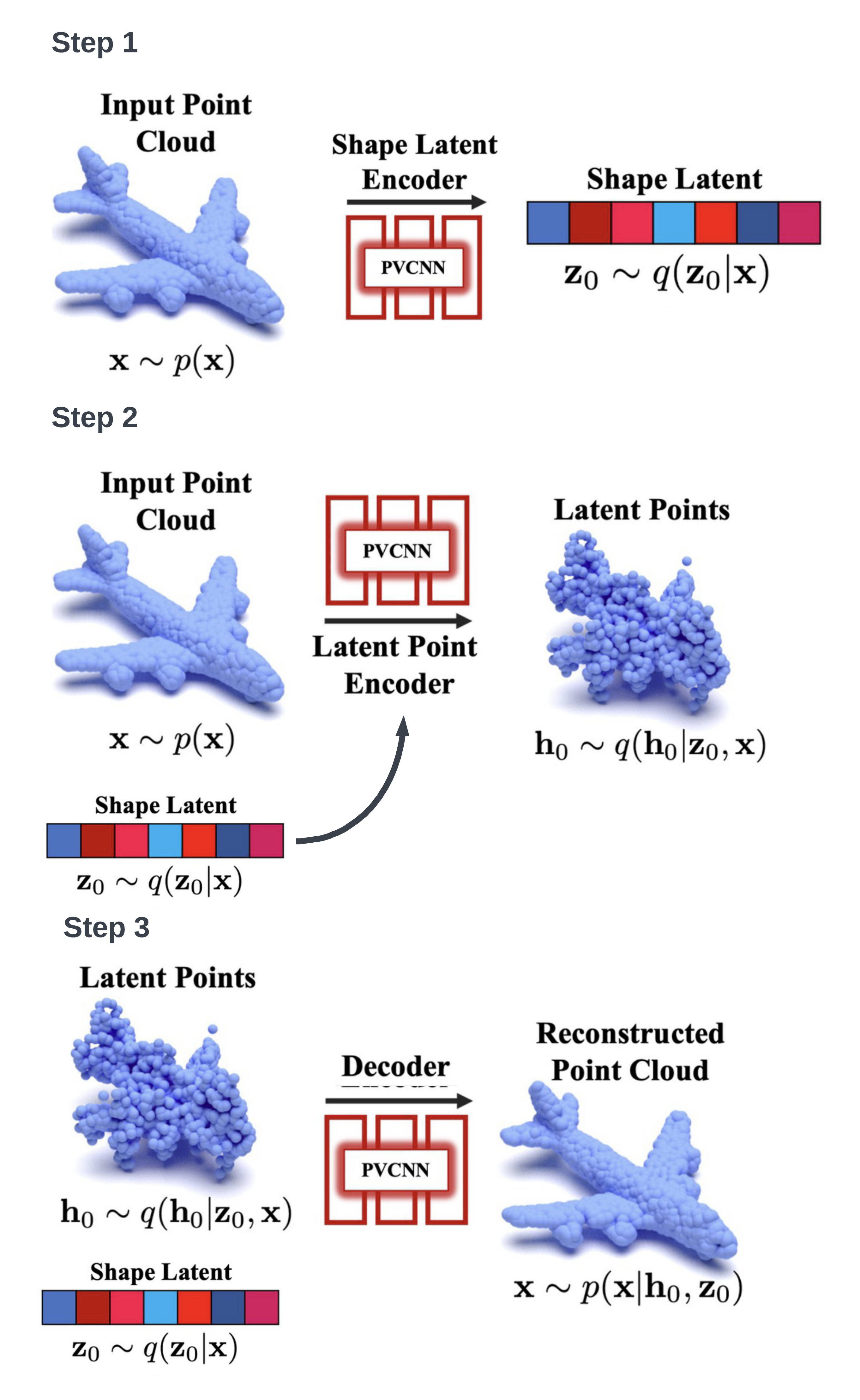
Stage 1: VAE

The VAE part, the encoding-decoding process has three steps:

1. Use a PVCNN to encode the whole point clouds into a latent vector (shape latent) $z_0\in {\mathbb{R}}^{D_z}$.
2. Concatenate shape latent with each point in the point cloud. Then use a PVCNN to map point clouds to latent "point clouds" $h_0\in {\mathbb{R}}^{3+D_h}$ in latent space.
3. Decoding from the concatenation of latent points and shape latent.

Stage 2: Diffusion

There are two diffusion processes involved since there are two latent vectors. Both diffusion processes start from standard normal distribution and mapped to shape latent vectors and point latent respectively.

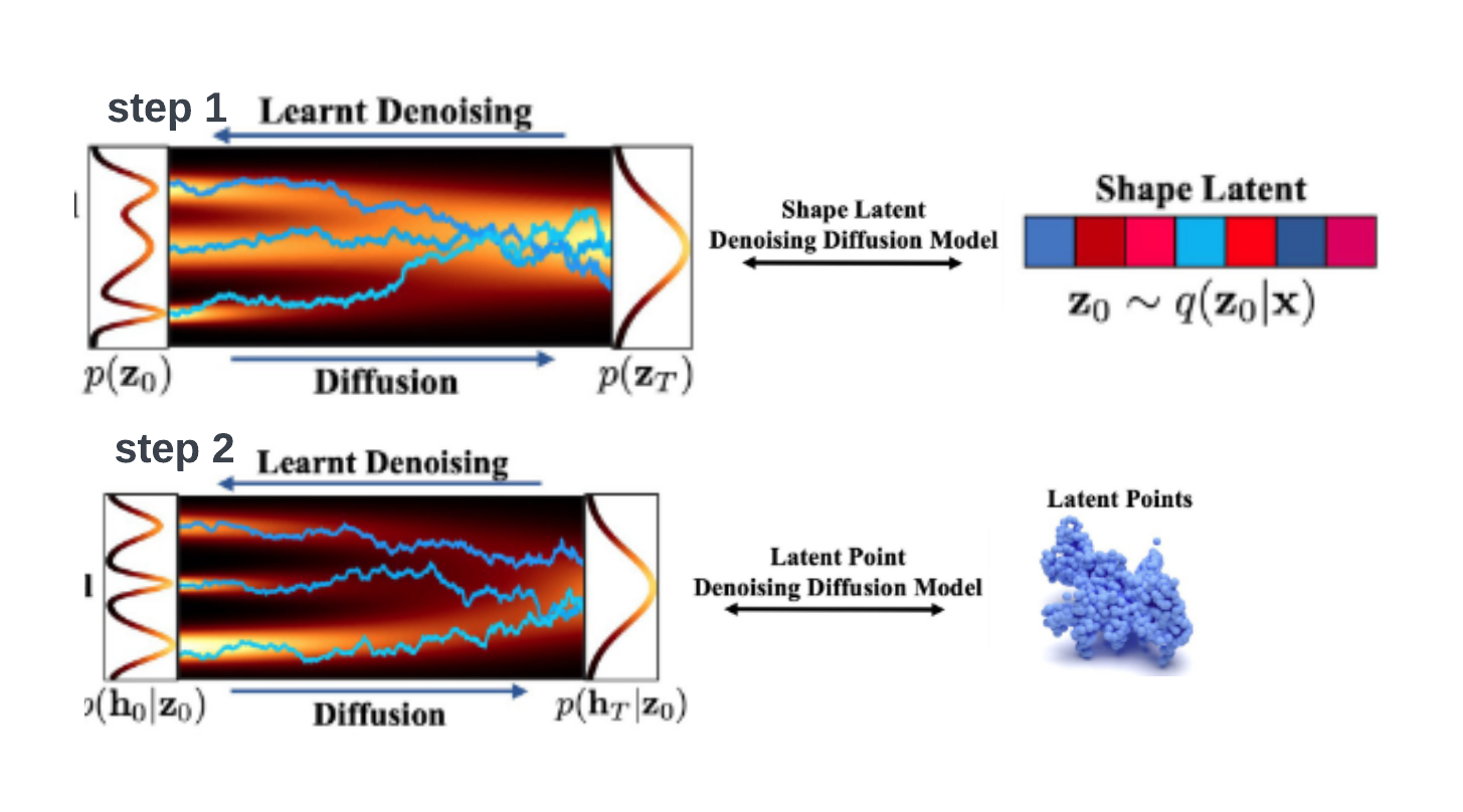
Sampling process

The sample generation process is consist of three steps:

1. Sample a vector from multivariate standard normal $z_T$ distribution and reverse diffused into shape latent $z_0$.
2. Sample a vector from multivariate standard normal $h_T$ and concatenate shape latent $z_0$ with each intermediate step $h_t$ and reversely diffused into point latents.

Training objective

During the training of VAE, LION is trained by maximizing a modified variational lower bound on the data log-likelihood with respect to the encoder and ecoder parameters $\varphi$ and $\xi$:

The priors $p(z_0)$ and $p(h_0)$ are $\mathcal{N}(0,I)$. During the training of diffusion models, the models are trained on embeddings and have VAE model fixed.

3D-LDM

Many previous works have discussed the limit of different methods of representing 3D shapes. Voxels are computationally and memory intensive and thus difficult to scale to high resolution; point clouds are light-weight and easy to process, but require a lossy post-processing step to obtain surfaces. Another form for representing shapes is SDF(signed distance function), it can be used to represent water-tight closed surface. In Nam et al., the paper proposed using coded shape DeepSDF and use diffusion model to generate code for shapes.

Formulation

Coded Shape SDF: This is a function $f_{\theta }(p,z)$ that maps a point $p$ and a latent representation of shapes $z$ to a signed distance(positive distance outside and negative distance inside). A set of shapes $\mathcal{S}$ can be represented with $f_{\theta }$ given a latent representation $z_i$:

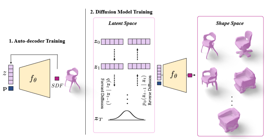
Training setup: DeepSDF has shown that $f_{\theta }$ can be trained efficiently in an encoder-less setup, called an auto-decoder, where each shape $S_i$ is explicitly associated with a latent vector $z_i$. These latent vectors are randomly assigned at first and learned during training process. Therefore, the algorithm is consist of two parts:

1. Auto-decoder for neural implicit 3D shapes.
2. Latent diffusion model for generating latent vector.

For the first part, the paper parameterizes the SDF with $\theta$ and $Z=\{z_i\}$ represents latent vectors. The objective function is following regularized reconstruction error:

Remarks:

1. The latent vectors $z_i$ was unknown before training and is randomly initialized. The training process learns both $\theta$ and $Z$ at the same time.
2. The training data is sampled through algorithm discussed in DeepSDF section 5. As implemented in DeepSDF, the data points are sampled within a certain box $[-\delta ,\delta ]$.

For the second part, the paper used the latent vectors $\{z_i\}$ generated during the training process in the first part as training data. The diffusion model follows the DDPM framwork and parameterized the model with ${ϵ}_{\varphi }(z^t,t)$. The paper claimed that they are following Ho et al. that it is more stably and efficiently to train the network to predict the total noise $z^t-z^0$. (I checked the DDPM paper and did not find related description. Personally, I think it is counter-intuitive to predict total noise and use it as step-wise noise.) In this framework, the training objective for this phase is:

Sampling process

The unconditional sampling step is exactly the same as DDPM. The reverse process is approximated by $p_{\varphi }(z^{t-1}\mid z^t)$ and is parameterized as a Gaussian distribution, where the mean ${\mu }_{\varphi }$ is defined as

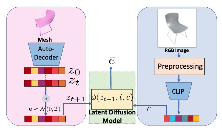
In the cases of conditional sampling, CLIP model is used to generate embedding for conditional information such as text and image. Then, concatenate latent vector with CLIP embedding and the reverse process mean ${\mu }_{\varphi }$ is modified into

SDFusion

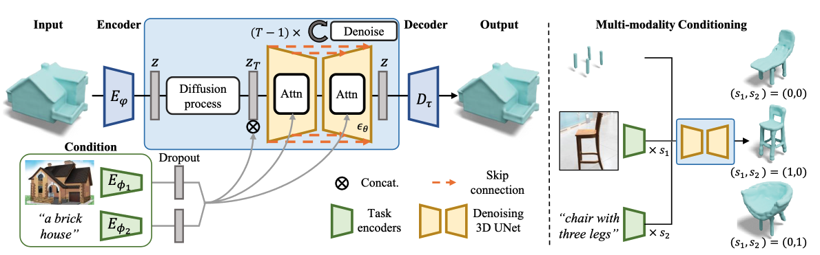
In 3D-LDM discussed above, the model architecture is an auto-decoder DeepSDF that learns the embedding during training. In Cheng et al., the author proposed an encoder-decoder model and, instead of using DeepSDF, used Truncated Signed Distance Field(T-SDF) to represent the shape. T-SDF is a simplified version of SDF and it limit or "truncate" the range of distances that we care about. It models a 3D shape with a volumetric tensor $X\in {\mathbb{R}}^{H\times W\times L}$. The algorithm in this paper is quite similar to previous ones and applied a latent diffusion model framework.

Formulation

The algorithm is consist of an auto-encoder for compression T-SDF data and a diffusion model in latent space.

3D shape Compression of SDF: The author leveraged a 3D variation of VA-VAE and, given an input shape in the form of T-SDF $X\in {\mathbb{R}}^{D\times D\times D}$, we have

In the above formulation, $E_{\varphi }\text{ and }{D}_{\tau }$ represent encoder and decoder between 3D space and latent space. VQ is the quantization step which maps the latent variable $z$ to the nearestt element in the codebook $\mathcal{Z}$. $E_{\varphi },D_{\tau },\text{ and }\mathcal{Z}$ are jointly trained.

Latent diffusion model for SDF: This part is exactly the same as DDPM. The paper use a time-conditional 3D UNet to approximate ${ϵ}_{\theta }$ and adopt the simplified objective function

References

(Citations removed)